No cost training to becoming a data scientist

most required skills for a data scientist position based on ReSkill's analyses of thousands of job posts and free resources to learn each skill:

1. Python

• Learn Python Programming From Scratch by Udemy
• Learn to program in Python by CodeCademy
• LearnPython.org interactive Python tutorial  

2. Machine Learning

• Machine learning online
• Operational Intelligence and Machine Data with Splunk  

3. R Language

• R Basics - R Programming Language Introduction by Udemy
• Introduction to R at DataCamp
• Learn R at Code school  

4. Big Data

• Big Data University
• Big Data and Hadoop Essentials by Udemy
• Basic overview of Big Data Hadoopby- Udemy  

5. Statistics

• Statistics One by Coursera
• Statistics and Probability
• Probability & Statistics  

6. Data Mining

• Data Mining and Web Scraping: How to Convert Sites into Data by Udemy
• Data Mining by Coursera  

7. SQL- Test your SQL skills

• Interactive Online SQL Training for Beginners
• Sachin Quickly Learns (SQL) - Structured Query Language by Udemy
• SQL Tutorial by w3schools

8. Java

• Learn Java: The Java Programming Tutorial For Beginners by Udemy
• Learn Java - Free Interactive Java Tutorial 
• Learn Java Programming From Scratch - Udemy  

Atomicity、Consistency、Isolation、Durability

1. Atomicity

一個交易（Transaction）是一個不可再分割的完整個體，它不是全部執行，就是全部不執行。以在 ATM 領錢來說，從你輸入密碼、到拿到錢、到帳戶扣帳為止，都必須正確執行完成。

2. Consistency

如果交易是全部執行，能讓資料庫從某個一致狀態，轉變到另一個一致狀態。以在 ATM 領錢來說，你領了 100 元，帳戶一定會少了 100 元。

3. Isolation

某交易執行期間所用的資料或中間結果，不容許其它交易讀取或寫入，直到此交易被確認（Commit，即：成功結束）為止；也就是說，它不應該被同時執行的其它交易所干擾。

以在 ATM 領錢來說，你領錢時，公司會計正好也在別家銀行辦理薪資轉帳，此時，若是你開始領錢的時間較早，那麼系統會將你的交易鎖定，直到你領錢的動作全部完成，才會再處理將你的薪資轉入你的戶頭的交易，反之亦然。

4.  Durability

一旦交易全部執行，且經過確認（Commit）後，此作業對資料庫所做的變更永遠有效，即使未來系統當機或毀損。也就是說，你提錢之後，帳戶少了 100 元就是少了 100 元，不會在經過一段時間後又恢復原來的金額。

Introduction to Random forest – Simplified

With increase in computational power, we can now choose algorithms which perform very intensive calculations. One such algorithm is “Random Forest”, which we will discuss in this article. While the algorithm is very popular in various competitions (e.g. like the ones running on Kaggle), the end output of the model is like a black box and hence should be used judiciously.

Before going any further, here is an example on the importance of choosing the best algorithm.

Importance of choosing the right algorithm

Yesterday, I saw a movie called ” Edge of tomorrow“.  I loved the concept and the thought process which went behind the plot of this movie. Let me summarize the plot (without commenting on the climax, of course). Unlike other sci-fi movies, this movie revolves around one single power which is given to both the sides (hero and villain). The power being the ability to reset the day.

Human race is at war with an alien specie called “Mimics”.  Mimic is described as a far more evolved civilization of an alien specie. Entire Mimic civilization is like a single complete organism. It has a central brain called “Omega” which commands all other organisms in the civilization. It stays in contact with all other species of the civilization every single second. “Alpha” is the main warrior specie (like the nervous system) of this civilization and takes command from “Omega”. “Omega” has the power to reset the day at any point of time.

Now, let’s wear the hat of a predictive analyst to analyze this plot. If a system has the ability to reset the day at any point of time, it will use this power, whenever any of its warrior specie die. And, hence there will be no single war ,when any of the warrior specie (alpha) will actually die, and the brain “Omega” will repeatedly test the best case scenario to maximize the death of human race and put a constraint on number of deaths of alpha (warrior specie) to be zero every single day. You can imagine this as “THE BEST” predictive algorithm ever made. It is literally impossible to defeat such an algorithm.

Let’s now get back to “Random Forests” using a case study.

 Case Study  

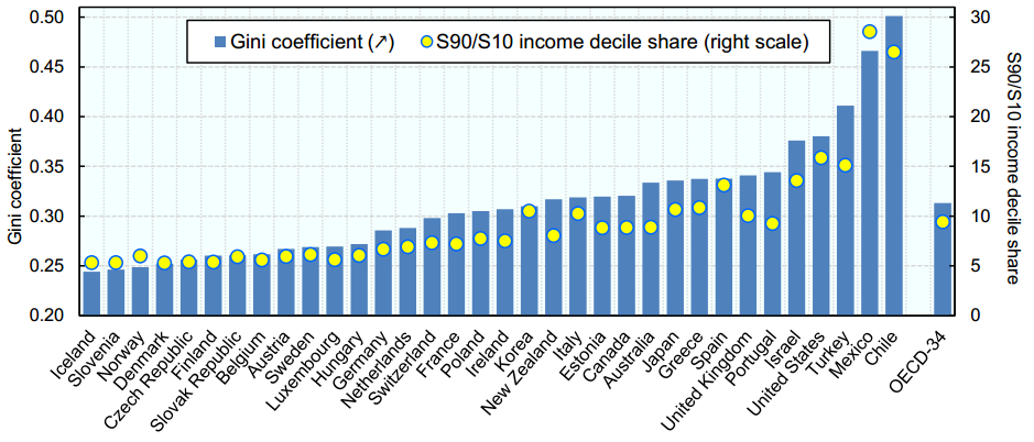
Following is a distribution of Annual income Gini Coefficients across different countries :

Mexico has the second highest Gini coefficient and hence has a very high segregation in annual income of rich and poor. Our task is to come up with an accurate predictive algorithm to estimate annual income bracket of each individual in Mexico. The brackets of income are as follows :

1. Below $40,000

2. $40,000 – 150,000

3. More than $150,000

Following are the information available for each individual :

1. Age , 2. Gender,  3. Highest educational qualification, 4. Working in Industry, 5. Residence in Metro/Non-metro

We need to come up with an algorithm to give an accurate prediction for an individual who has following traits:

1. Age : 35 years , 2, Gender : Male , 3. Highest Educational Qualification : Diploma holder, 4. Industry : Manufacturing, 5. Residence : Metro

We will only talk about random forest to make this prediction in this article.

 The algorithm of Random Forest 

Random forest is like a bootstrapping algorithm with Decision tree (CART) model. Say, we have 1000 observation in the complete population with 10 variables. Random forest tries to build multiple CART model with different sample and different initial variables. For instance, it will take a random sample of 100 observation and 5 randomly chosen initial variables to build a CART model. It will repeat the process (say) 10 times and then make a final prediction on each observation. Final prediction is a function of each prediction. This final prediction can simply be the mean of each prediction.

 Back to Case study 

Disclaimer : The numbers in this article are illustrative

Mexico has a population of 118 MM. Say, the algorithm Random forest picks up 10k observation with only one variable (for simplicity) to build each CART model. In total, we are looking at 5 CART model being built with different variables. In a real life problem, you will have more number of population sample and different combinations of  input variables.

Salary bands :

Band 1 : Below $40,000

Band 2: $40,000 – 150,000

Band 3: More than $150,000

Following are the outputs of the 5 different CART model.

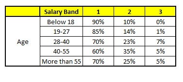
CART 1 : Variable Age

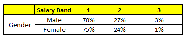
CART 2 : Variable Gender

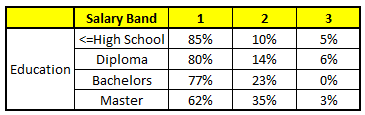
CART 3 : Variable Education

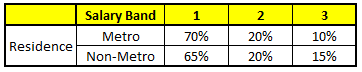
CART 4 : Variable Residence

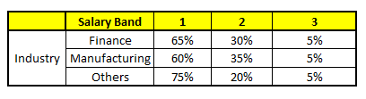
CART 5 : Variable Industry

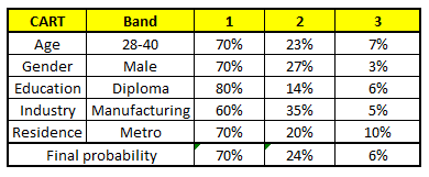
Using these 5 CART models, we need to come up with singe set of probability to belong to each of the salary classes. For simplicity, we will just take a mean of probabilities in this case study. Other than simple mean, we also consider vote method to come up with the final prediction. To come up with the final prediction let’s locate the following profile in each CART model :

1. Age : 35 years , 2, Gender : Male , 3. Highest Educational Qualification : Diploma holder, 4. Industry : Manufacturing, 5. Residence : Metro

For each of these CART model, following is the distribution across salary bands :

The final probability is simply the average of the probability in the same salary bands in different CART models. As you can see from this analysis, that there is 70% chance of this individual falling in class 1 (less than $40,000) and around 24% chance of the individual falling in class 2.

 End Notes 

Random forest gives much more accurate predictions when compared to simple CART/CHAID or regression models in many scenarios. These cases generally have high number of predictive variables and huge sample size. This is because it captures the variance of several input variables at the same time and enables high number of observations to participate in the prediction. In some of the coming articles, we will talk more about the algorithm in more detail and talk about how to build a simple random forest on R.

Comparing a CART model to Random Forest

http://www.analyticsvidhya.com/blog/2014/06/comparing-cart-random-forest-1/

http://www.analyticsvidhya.com/blog/2014/06/comparing-random-forest-simple-cart-model/

Powerful Guide to learn Random Forest (with codes in R & Python)

Introduction

Random Forests is panacea to all data science problems!

Random Forest models have risen significantly in their popularity – and for some real good reasons. They can be applied quickly to any data science problems to get first set of benchmark results. They are incredibly powerful and can be implemented quickly out of the box.

Please note that I am saying first set of results and not all results. Because they have a few limitations as well. In this article, I’ll introduce you to the most interesting aspects of applying Random Forest in your predictive models.

Table of Contents

1. History of Random Forest
2. What is Random Forest?
3. How to implement Random Forest in Python and R?
4. How does it work?
5. Pros and Cons associated with Random Forest
6. How to tune Parameters of Random Forest?
7. Practice Problem

History of Random Forest

The history began way back in 1980s. This algorithm was a result of incessant team work by Leo Breiman, Adele Cutler, Ho Tin Kam, Dietterich, Amit and Geman. Each of them played a significant role in early development of random forest. The algorithm for actuating a random forest was developed by Leo Breiman and Adele Cutler. This algorithm is register in their (Leo and Adele) trademark. Amit, Gemen, Ho Tim Kam, independently introduced the idea of random selection of features and using Breiman’s ‘Bagging’ idea constructed this collection of decision trees with controlled variance. Later, Deitterich introduced the idea of random node optimization.                                                                                                                                                  Leo Breiman

What is Random Forest?

Random Forest is a versatile machine learning method capable of performing both regression and classification tasks. It also undertakes dimensional reduction methods, treats missing values, outlier values and other essentialsteps of data exploration, and does a fairly good job. It is a type of ensemble learning method, where a group of weak models combine to form a powerful model.

In Random Forest, we grow multiple trees as opposed to a single tree in CART model (see comparison between CART and Random Forest here, part1 and part2). To classify a new object based on attributes, each tree gives a classification and we say the tree “votes” for that class. The forest chooses the classification having the most votes (over all the trees in the forest) and in case of regression, it takes the average of outputs by different trees.

Python & R implementation:

Random forests have commonly known implementations in R packages and Python scikit-learn. Let’s look at the code of loading random forest model in R and Python below:

Python

#Import Library
from sklearn.ensemble import RandomForestClassifier #use RandomForestRegressor for regression problem
#Assumed you have, X (predictor) and Y (target) for training data set and x_test(predictor) of test_dataset
# Create Random Forest object
model= RandomForestClassifier(n_estimators=1000)
# Train the model using the training sets and check score
model.fit(X, y)
#Predict Output
predicted= model.predict(x_test)

R Code

library(randomForest)
x <- cbind(x_train,y_train)
# Fitting model
fit <- randomForest(Species ~ ., x,ntree=500)
summary(fit)
#Predict Output 
predicted= predict(fit,x_test)

Now that you know how to run random forest (I bet, that wasn’t difficult), let’s understand how random forest algorithm works?

How Random Forest algorithm works?

In Random Forest, each tree is planted & grown as follows:

1. Assume number of cases in the training set is N. Then, sample of these N cases is taken at random but with replacement. This sample will be the training set for growing the tree.
2. If there are M input variables, a number m<M is specified such that at each node, m variables are selected at random out of the M. The best split on these m is used to split the node. The value of m is held constant while we grow the forest.
3. Each tree is grown to the largest extent possible and  there is no pruning.
4. Predict new data by aggregating the predictions of the ntree trees (i.e., majority votes for classification, average for regression).

To understand more in detail about this algorithm using a case study, please read this article “Introduction to Random forest – Simplified“.

Pros and Cons of Random Forest

Pros:

• As I mentioned earlier, this algorithm can solve both type of problems i.e. classification and regression and does a decent estimation at both fronts.
• One of benefits of Random forest which excites me most is, the power of handle large data set with higher dimensionality. It can handle thousands of input variables and identify most significant variables so it is considered as one of the dimensionality reduction methods. Further, the model outputs Importance of variable, which can be a very handy feature. Look at the below image of variable importance from currently Live Hackathon 3.x.
  
• It has an effective method for estimating missing data and maintains accuracy when a large proportion of the data are missing.
• It has methods for balancing errors in datasets where classes are imbalanced.
• The capabilities of the above can be extended to unlabeled data, leading to unsupervised clustering, data views and outlier detection.
• Random Forest involves sampling of the input data with replacement called as bootstrap sampling. Here one third of the data is not used for training and can be used to testing. These are called the out of bag samples. Error estimated on these out of bag samples is known as out of bag error. Study of error estimates by Out of bag, gives evidence to show that the out-of-bag estimate is as accurate as using a test set of the same size as the training set. Therefore, using the out-of-bag error estimate removes the need for a set aside test set.

Cons:

• It surely does a good job at classification but not as good as for regression problem as it does not give continuous output. In case of regression, it doesn’t predict beyond the range in the training data, and that they may over-fit data sets that are particularly noisy.
• Random Forest can feel like a black box approach for statistical modelers – you have very little control on what the model does. You can at best – try different parameters and random seeds!

How to Tune Parameters of Random Forest?

Till now, we have looked at the basic random forest model, where we have used the default values of various parameters except n_estimators=1000. Here we will look at the different parameters, its importance and methods to tune. Below is the syntax of Random Forest model in python scikit-learn.

class sklearn.ensemble.RandomForestClassifier(n_estimators=10, criterion='gini', max_depth=None,min_samples_split=2, min_samples_leaf=1, min_weight_fraction_leaf=0.0, max_features='auto', max_leaf_nodes=None,bootstrap=True, oob_score=False, n_jobs=1, random_state=None, verbose=0, warm_start=False, class_weight=None)

Follow definition of these metrics here.

These parameters play a vital role in adjusting the accuracy of your random forest model. The intelligent use of these metrics improve the power of model significantly. To understand this aspect in more detail, you can refer this article “Tuning parameters of random forest model“.

Practice Problem

In currently Live, Hackathon 3.x – Predict customer worth for Happy Customer Bank, a binary classification problem is given. This problem has 24 input variables( mix of both categorical and continuous variables). Input variables have missing values, outlier values and unbalanced distribution of numerical variables.

After we’ve finished hypothesis generation and basic data exploration, my next step is to use a classification algorithm. I can choose from various classification algorithms like Logistic, SVM, Random Forest and many others. But here, I’ll compare the performance of logistic regression and random forest model.

For initial model, I have not done any feature engineering and data cleaning. Let’s look at the output of these three models and their relative performance:

Step-1: Initial steps of importing libraries and reading data:

import pandas as pd
import numpy as np
from sklearn.ensemble import RandomForestClassifier
from sklearn.linear_model import LogisticRegression
from sklearn import preprocessing
from sklearn.metrics import roc_curve, auc

number = preprocessing.LabelEncoder()

train=pd.read_csv('C:/Users/Analytics Vidhya/Desktop/Hackathon3.x/Final_Files/Train.csv')

Step-2: Convert categorical variable to numpy arrays and fill NaN values to zero.

def convert(data):
number = preprocessing.LabelEncoder()
data['Gender'] = number.fit_transform(data.Gender)
data['City'] = number.fit_transform(data.City)
data['Salary_Account'] = number.fit_transform(data.Salary_Account)
data['Employer_Name'] = number.fit_transform(data.Employer_Name)
data['Mobile_Verified'] = number.fit_transform(data.Mobile_Verified)
data['Var1'] = number.fit_transform(data.Var1)
data['Filled_Form'] = number.fit_transform(data.Filled_Form)
data['Device_Type'] = number.fit_transform(data.Device_Type)
data['Var2'] = number.fit_transform(data.Var2)
data['Source'] = number.fit_transform(data.Source)
data=data.fillna(0)
return data
train=convert(train)

Step-3: Split the data set to train and validate

train['is_train'] = np.random.uniform(0, 1, len(train)) <= .75
train, validate = train[train['is_train']==True], train[train['is_train']==False]

Step-4: Build Logistic and look at the roc_auc (evaluation metric of this challenge)

lg = LogisticRegression()
lg.fit(x_train, y_train)

Disbursed_lg=lg.predict_proba(x_validate)

fpr, tpr, _ = roc_curve(y_validate, Disbursed_lg[:,1])
roc_auc = auc(fpr, tpr)
print roc_auc

Output: 0.535441187235

Step-5: Build Random and look at the roc_auc

rf = RandomForestClassifier()
rf.fit(x_train, y_train)
disbursed = rf.predict_proba(x_validate)
fpr, tpr, _ = roc_curve(y_validate, disbursed[:,1])
roc_auc = auc(fpr, tpr)
print roc_auc

Output: 0.614586623764

Step-6: Build Random Forest with n_estimtors=1000 and look at the roc_auc

rf = RandomForestClassifier(n_estimators=1000)
rf.fit(x_train, y_train)
disbursed = rf.predict_proba(x_validate)
fpr, tpr, _ = roc_curve(y_validate, disbursed[:,1])
roc_auc = auc(fpr, tpr)
print roc_auc

Output: 0.824606785363

By looking at above models, it is clear that random forest with tuned parameter has better results than other two. You can further improve the model power by tuning other parameters also. Above, we have not done any feature engineering, you can populate featured variable(s), treat missing or outlier values, combine multiple models and generate a powerful ensemble methods. This competition is Live till 11th September 2015, therefore, I can’t discuss more as it will violate T&C of competition.

End Note

In this article, we looked at one of most common machine learning algorithm Random Forest followed by its pros & cons, method to tune parameters and explained & compared it using a practice problem. I would suggest you to use random forest and analyse the power of this model by tuning the parameters.